Blog

How do we decide when to buy or sell a stock option? I’m trying to dedicate a blog post to the stuff I learned reading a few interesting papers about ML for portfolio hedging and optimization.

Technical vs Fundamental analysis

There are two different philosophies shared among the trader community ¹. One is the Fundamental analysis that focuses on evaluating the intrinsic value of an asset based on underlying economic and financial factors. This approach involves examining company financials, such as revenue, earnings, profit margins, and debt levels, to understand the health and prospects of a business. For instance, a strong balance sheet or consistent revenue growth might indicate a company worth investing in. It also considers macroeconomic indicators like interest rates, inflation, and GDP growth, which can influence industries and markets.

In contrast, technical analysis focuses on studying price movements and patterns to predict future price behavior. This approach centers on analyzing charts and trends to identify market directions, such as uptrends, downtrends, or consolidations. It employs indicators like the Moving Average Convergence Divergence (MACD), Relative Strength Index (RSI), and Bollinger Bands to assess momentum, volatility, and overbought or oversold conditions.

How to decide which stock?

According to technical analysis, we are looking for patterns in price movements and indicators. People who perform this type of analysis are often referred to as chartists ¹.

A sign of an upward trend is called bullish, indicating optimism and rising prices. Conversely, a sign of a downward trend is called bearish, signaling pessimism and falling prices. 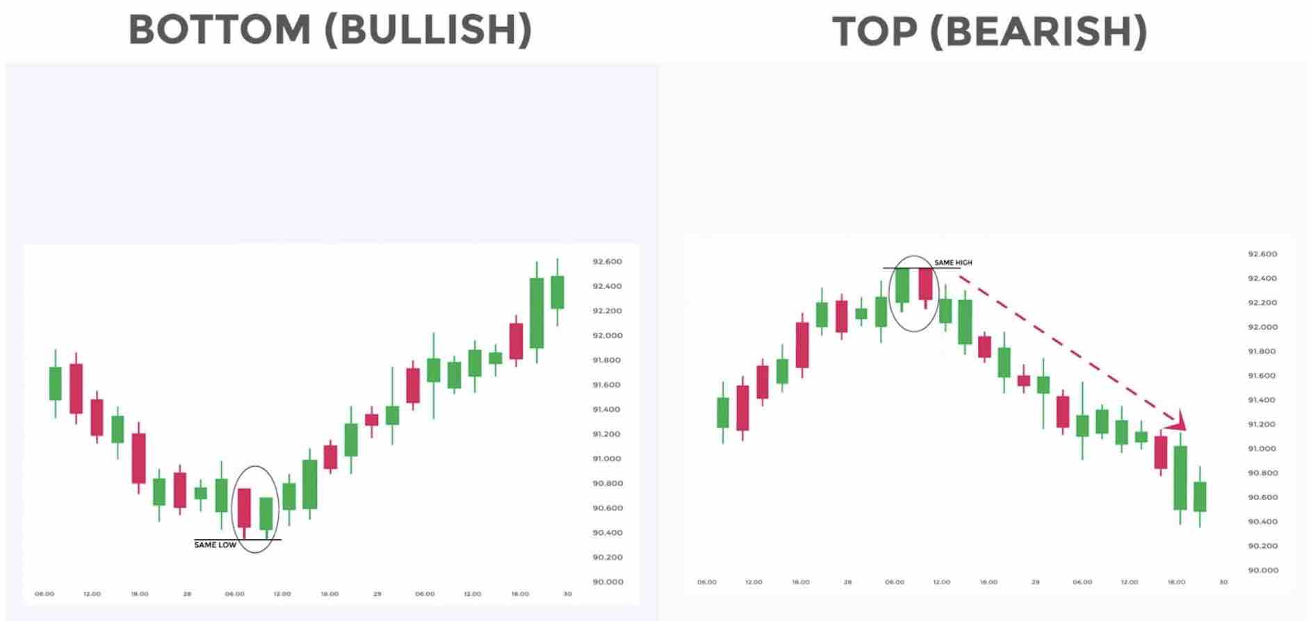(Taken from ²)

When deciding which stock to trade or invest in, traders and investors rely on various metrics to identify trends, assess momentum, and evaluate market conditions. These metrics serve as tools to decipher market behavior and reduce uncertainty in decision-making. By analyzing these indicators, traders aim to predict the direction of stock prices and strategically plan their entry and exit points.

The essence of using technical indicators lies in answering critical questions: Is the stock price likely to rise or fall? Is the asset overbought or oversold? Are we entering a period of increased volatility? These insights are vital for both short-term traders seeking quick gains and long-term investors aiming for sustained growth.

We have several metrics to choose from:

• Moving Average Convergence Divergence (MACD) measures the relationship between two exponential moving averages (EMAs) of a stock’s price. We could calculate MACD = 12-day EMA - 26-day EMAs and if its larger or lower than 9-day EMA it could indicate a bullish or bearish signal.
• The Relative Strength Index (RSI) is a momentum oscillator that evaluates the speed and magnitude of recent price changes to determine whether an asset is overbought or oversold. It is calculated using the formula: $$RSI = 100 - \frac{100}{1+\frac{Average Gain}{Average Loss}}$$ Typically a $RSI > 70$ indicates a potential reversal downward and $RSI < 30$ a potential reversal upward.
• Bollinger Bands are a popular volatility indicator that consists of three lines: a Simple Moving Average (SMA) and two bands above and below it at a distance of two standard deviations.

Instead of manually looking at charts, we could for instance check if any stock lately emitted a signal according to:

• MACD: Large historic price move
• Bollinger Band breach
• RSI potential upward trend coming

In Python we could use Yahoo Finance to get a grip on historic stock prices.

 1
 2
 3
 4
 5
 6
 7
 8
 9
10
11
12
13
14
15
16
17
18
19
20
21
22
23
24
25
26
27
28

import yfinance as yf

for ticker in msci_world_tickers:
    print(f"Processing {ticker}...")
    try:
        # Fetch historical stock data
        df = yf.download(ticker, period="300d", interval="1d")
        large_price_move = abs(prelatest_row["Close"].item() - latest_row["Close"].item()) > 4 * latest_row["200_Variance"].item()
        rsi_signal = latest_row["RSI"].item() < 15 
    
        bollinger_breach = latest_row["Close"].item() > latest_row["Upper_Band"].item()
                            or latest_row["Close"].item() < latest_row["Lower_Band"].item()
        if large_price_move or rsi_signal or bollinger_breach:
            filtered_stocks.append({
                "Stock": ticker,
                "Date": latest_row.name.date(),
                "Close": latest_row["Close"].item(),
                "Close_pre": prelatest_row["Close"].item(),
                "Variance": latest_row["200_Variance"].item(),
                "RSI": latest_row["RSI"].item(),
                "MACD": latest_row["MACD"].item(),
                "Signal": latest_row["Signal"].item(),
                "Upper_Band": latest_row["Upper_Band"].item(),
                "Lower_Band": latest_row["Lower_Band"].item(),
                "event": ("Oversold," if rsi_signal else "") 
                         + ("Bound breach," if bollinger_breach else "")
                         + ("large price move" if large_price_move else "")
            })

We could even loop over all stocks from a market regularly and check if there is an interesting trend/anomaly happening.

(Complete code: https://gist.github.com/anon767/b2598327451557bd64d3bbd71a9e731b)

Background

The basic idea when trading options in the stock market is to buy a call option to benefit from price increases or a put option to benefit from price decreases. European vanilla option gives the buyer the right, but not the obligation, to buy (call) or sell (put) an underlying asset at a specific strike price $K$ at maturity $T$. The payoff is $(S_T - K)^+$ in case of a call where $S_T$ is the stock price at maturity. The process of identifying profitable opportunities revolves around predicting how the price of the underlying asset (stock) might evolve over time.

There are several ways to price options, with the Black-Scholes model being one of the most widely used techniques³: $$C(S,t) = SN(d_1) - Ke^{-r(T-t)}N(d_2)$$ This formula calculates the price of a call option where $N$ is the cumulative distribution function of a standard normal distribution, $S$ the current stock price, $T-t$ the time until maturity, $r$ is the risk-free annual interest rate and $\sigma$ is the volatility of the asset.

$d_1$ and $d_2$ build the solution to the Black-Scholes PDE: $$d_1 = \frac{log(S/K)+(r-q_\sigma^2/2)(T-t)}{(\sigma\sqrt{T-t)}}$$ $$d_1 = d_1-\sigma\sqrt{T-t}$$

The Black-Scholes model determines the fair price of a call option based on the underlying asset’s volatility and the prevailing risk-free interest rate ⁴. Volatility reflects the risk associated with the asset: higher volatility indicates greater uncertainty, with more significant potential price swings in either direction. The risk-free rate is the potential interest you get from some investment instrument that has zero risk. Riskier investments need to offer a higher return to compensate for additional uncertainty. Later, we will refer to the return on risk-free interest as $R^f$.

While the Black-Scholes model is instrumental in determining the fair price of options, it inherently relies on the characteristics of the underlying stock, such as its current price, volatility, and expected future movements. This raises a fundamental question: how do we determine the true value of the stock itself?

Risk and Reward

While understanding the intrinsic value of a stock is crucial for identifying potential investment opportunities, it is only one piece of the broader puzzle. Successful investing requires not only selecting individual stocks but also constructing a portfolio that balances risk and reward. This involves understanding how different assets interact within a portfolio and employing strategies to manage volatility and optimize returns.

We already have spoken about reward and stock returns, that is just $(S_T - K)^+$ in case of a call option. The volatility is obviously considered the risk. But what can we do to reduce the risk of one stock? One effective strategy is hedging, which involves taking a position in a related asset to offset potential losses. For example, if you own a stock and are concerned about its price dropping, you might buy a put option on that stock to limit your downside risk. Alternatively, you could pair it with another stock or financial instrument that tends to move inversely, balancing the impact of adverse market movements.

A portfolio is a collection of financial assets (e.g., stocks, bonds, derivatives) where each asset has a specific allocation (weight): $P = [p_1,p_2,…,p_n]$ while $\sum_1^n p_i = 1$ We can calculate the return of $P$ by: $R_P = \sum p_iS_i(t)$ and the variance $\Sigma_P = \sigma^2_P = \sum_i^n\sum_j^n(p_ip_jCov(R_i,R_j))$ .With $Cov()$ being the covariance between to asset returns.

A common portfolio strategy for traders is the 70/30 rule, where 70% of the portfolio is allocated to stable investments, such as ETFs that track broad market indices, and the remaining 30% is directed towards higher-risk, higher-reward opportunities like emerging markets.

Portfolio Optimization

Harry Markowitz introduced the modern portfolio theory. At the heart of this, we aim to find the efficient frontier, which represents the set of optimal portfolios that offer the maximum expected return for a given level of risk or the minimum risk for a given level of return. $$P^T\Sigma_P P-qR^TP$$ This tells us the weights for our portfolio to minimize risk given a risk tolerance $q \geq 0$ and maximize the expected return.

Markowitz found out that we can also redefine it as a optimization goal: We could find a maximum return portfolio for a given risk.

$$\max_P R(P)$$ $$s.t.$$ $$\phi_i(P) \leq c_i \forall i$$

We want to optimize $P$ such that the reward is maximized, and the smaller than a given risk.

We could also minimize the risk which is the dual of the former optimization goal:

$$\min_P \phi_i(P) $$ $$s.t.$$ $$R(P) \geq \mu$$ $$\sum_i^n p_i = 1$$

Where $\mu$ is the expected return of the portfolio.

I replaced the risk measurement from Markovitz $\Sigma_P$ with a function $\phi_i(P)$. This aligns with the riskfolio Python lib. There are around 20 risk measurements available and three ways to calculate the return (arithmetic return according to Markovitz, approximate logarithmic return, exact logarithmic return). Why do there exist different Risk measurements and return definitions?

Well, risk is a multifaceted concept, and different risk measurements capture various aspects of uncertainty. Markowitz’s definition of risk, using volatility, equally weights upward and downward volatility. However, downward volatility is more detrimental to an investor’s call option than upward movements. This is why alternative measures, such as semi-standard deviation, exist to focus specifically on downside risk. Additionally, sometimes we need to account more strongly for tail and worst-case risks, which is where measures like Maximum Drawdown come into play. For more complex modeling, we may want to exponentially discount returns over time to reflect their diminishing importance in the future.

But how can we solve such optimization tasks?

Solvers

There are different optimization problems that can be differently classified e.g. as Linear vs Non-Linear, Discrete vs Continuuous, Deterministic vs Stochastic, … Different solvers exist for different problems. Some of them like the MOSEK suggested by the Riskfolio lib are commercial and not quite cheap. However, some problems can be solved easily. In the next chapter Id like to talk a bit about optimization methods and a few common algorithms to solve optimization problems. Finally, we take a look at ML for portfolio optimization.

Simplex method

For Linear problems we can use algorithms like the simplex method with an example implementation here: https://gist.github.com/anon767/a1996c7c541be9d0f6538c67bcbda996. The simplex method operates on the feasible region, which is a convex polytope formed by the constraints. Each corner (vertex) of the polytope represents a basic feasible solution. The algorithm moves from one vertex to an adjacent vertex, improving the objective function at each step, until it reaches the vertex that maximizes (or minimizes) the objective function.

Whenever the objective function and constraints depend linearly on the parameters, the simplex method is a good starting point. However, the Markovitz portfolio optimization for example is a quadratic problem.

Lagrange Multipliers

We can use Lagrange Multipliers to solve the Markovitz Portfolio optimization problem. Lagrange multipliers transform a constrained optimization problem into an unconstrained one by incorporating the constraints into the objective function.

Lets say we have: $$\min_P P^T\Sigma P$$

Subject to: $$R(P) = P^TR \geq \mu, \sum_i^n p_i = 1$$

We can define Lagrangian functions by $$L(P, \lambda_1, \lambda_2) = P^T\Sigma P - \lambda_1(P^TR-\mu) - \lambda_2((\sum_i^n p_i) - 1)$$

Where $\lambda_1$ is the Lagrange multiplier for the first constraint and $\lambda_2$ for the second. To find the optimal solution we can take the derivatives and set them to zero:

$$\frac{\partial L}{\partial P} = 2\Sigma P- \lambda_1 R - \lambda_2 = 0$$ $$\frac{\partial L}{\partial \lambda_1} =P^TR-\mu= 0$$ $$\frac{\partial L}{\partial \lambda_2} = (\sum_i^n p_i) - 1 = 0$$

Convex Optimization

Convex optimization is a significant branch of optimization theory, focusing on problems defined on convex sets with convex functions ⁵. To comprehend convex optimization, we first need to understand two fundamental concepts: Convex Sets and Convex Functions.

In Euclidean space, a set is called convex if the line segment between any two points within the set lies entirely within the set:

Formally, a set $C$ is convex if, for any $x, y \in C$ and any $\theta$ satisfying $0 \leq θ \leq 1$, the point $\theta x + (1 — θ)y$ is also in $C$. A function $f$ defined on a convex set $D$ is called a convex function if, for all $x, y \in D$ and $0 \leq θ \leq 1$, it holds that $f(\theta x + (1 — θ)y) \leq \theta f(x) + (1 — \theta)f(y)$ Intuitively, this means the chord line of the function always lies above or on the graph of the function.

Convex problems ensure that any local minimum is also a global minimum. This property avoids the pitfalls of non-convex optimization, where algorithms can get stuck in suboptimal solutions.

Stochastic Gradient Descent

Lets say we have a function that calculates the quality of a portfolio given its weights. In our example $P$ is our set of parameters and a quality, aka, loss function can be defined as: $$L(P)=λP^T\Sigma P − (1−λ)R^T P$$

where $\lambda$ quantizes the weight of importance for return vs. risk. Given an initial $P_t$ we want to iteratively update it to obtain a better $P_{t+1}$.

$$P_{t+1} = P_t - \eta \nabla_PL(P_t)$$

Where $P_t$ are the portfolio weights at iteration $t$, $\eta$ is a learning rate which is required for non-convex optimization problems and $$\nabla L(P_t) = 2\lambda\Sigma P_t - (1 - \lambda) R$$ which defines the gradient for the loss function which points toward the minimum.

Iterating means actually descending to a local minimum (global minimum in a convex problem). A potential stopping criteria might be a convergence of $P$ by $|P_{t+1} - P_t| \le \epsilon$.

Interior Point Method

A known solver for convex problems is the interior point method which takes a minimization problem with a convex loss function and inequality constraints. Given a constraint $g(x) \leq 0$, we can define a barrier function: $$\Phi(x) = - \sum_i^m ln(-g_i(x)))$$ This term becomes very large (tends to infinity) as x approaches the boundary.

Then we can basically use newtons method to solve:

$$\min_x f(x) + \frac{1}{t_k}\Phi(x)$$

With

$$x_{k+1} = x_k - H^{-1}\nabla F(x_k)$$

Where $F(x) = f(x) + \frac{1}{t_k}\Phi(x)$, $\nabla F(x)$ is the gradient and $H = \nabla^2 F(X)$ the Hessian matrix or the second order derivative. We can have the following stopping criteria: $$||\nabla f(x) + \nabla \Phi(x)|| \le \epsilon$$

Second order optimization functions

Second-order optimizers leverage the curvature (second derivatives) of the loss function to make more informed updates. We already have seen a second order derivative defined by the Hessian matrix $H = \nabla^2f(x)$ in the Newton method. However, its very computational costly and requires $O(n^2)$ space for the parameters. Today we tend to see first-order optimizing algorithms that approximate second-order behaviour adaptively.

RMSProp approximates the second-order curvature of the loss function by tracking the squared gradients over time: $$g_t = \nabla f(x)$$ $$v_t = \beta v_{t-1} + (1-\beta)g_t^2$$ where $v_t$ is the weighted moving average with a decay rate of $\beta$.

The update rule is then defined as: $$x_{t+1} = x_t - \eta \frac{g_t}{\sqrt(v_t + \epsilon)}$$

Adam for instance uses first and second moment (mean and variance) of the first-order gradients ⁶.

Hedging with Deep Learning

Neural networks are highly flexible tools that can approximate solutions for both convex and non-convex problems due to their universal approximation capability ⁷. Even though most of the market processes to be analysed possess the Markov property according to the Efficient Market Hypothesis (EMH), we still require our model to be able to take into account all of the actions that took place in the past ⁸.

Let $X \in \mathbb{R}^{T x d}$ be the historical stock data of daily closing prices. $T$ is the number of trading days, $d$ the number of stocks in $P$ and $x_{t,i}$ the price of stock $i$ at time $t$. The neural network is a function of $$P = F_\theta(x)$$

We have $m$ layers with a ReLU activation function and a softmax output layer to enforce the constraint $\sum_i p_i = 1$: $$p_i = \frac{exp(z_i)}{\sum_j^d exp(z_j)}$$

The network is trained to minimize a loss function $L$, which represents the portfolio’s risk-return measure. We define different objective functions where MV is quadratic programming problem, EVaR being a exponential cone problem and CDaR a classic linear programming problem.

• Conditional Drawdown at Risk: $CDaR = \mathbb{E} \left[ max_{t \in [0, \alpha T]} (1 - \frac{V}{\max_{s \leq t} V_s})\right]$ with $V_t$ being portfolio value at $t$.

The loss function for CDaR minimizes the average of the worst-case drawdowns over a specified confidence level $\alpha$: $$L_{\text{CDaR}} = \frac{1}{\alpha} \sum_{t \in T_\alpha} \max \left( 0, 1 - \frac{V_t}{\max_{s \leq t} V_s} \right)$$

1
2
3
4
5
6
7
8

def cdar_loss(returns, weights, alpha=0.95):
    portfolio_returns = torch.matmul(returns, weights)
    portfolio_values = torch.cumsum(portfolio_returns, dim=0) 
    max_values = torch.cummax(portfolio_values, dim=0)[0]
    drawdowns = 1 - (portfolio_values / max_values)
    sorted_drawdowns = torch.sort(drawdowns, descending=True)[0]
    worst_drawdowns = sorted_drawdowns[:int(len(sorted_drawdowns) * (1 - alpha))]
    return worst_drawdowns.mean()

• Entropic Value at Risk: $L_{EVaR} = \inf_{\lambda > 0} \left[ \lambda \ln \mathbb{E} \left[ \exp\left( -\frac{R_P}{\lambda} \right) \right] \right]$ minimizes the tail risk of the portfolio by focusing on extreme outcomes, using an exponential cone formulation.

1
2
3
4
5

def evar_loss(returns, weights, risk_aversion=0.1):
    portfolio_returns = torch.matmul(weights, returns.T)
    lambda_param = risk_aversion
    exp_term = torch.exp(-portfolio_returns / lambda_param)
    return lambda_param * torch.log(torch.mean(exp_term))

• The MV loss function $L_{MV} = \lambda P^T\Sigma P - (1 - \lambda) R^TP$ minimizes the portfolio variance while balancing it with the expected return.

1
2
3

def mean_variance_loss(returns, weights, cov_matrix, risk_aversion=0.5):
    portfolio_return = torch.matmul(weights, returns.mean(dim=0))
    return risk_aversion * cov_matrix - (1 - risk_aversion) * portfolio_return

CDaR, which minimizes drawdowns, is ideal for risk-averse investors focused on preserving capital and reducing extreme losses. EVaR caters to those concerned with tail risks, striking a balance between managing extreme outcomes and achieving higher returns, making it suitable for moderately risk-averse investors. Meanwhile, MV optimization balances risk and return, making it a versatile choice for diversified investors seeking steady growth without prioritizing extremes.

The full problem becomes: $\min_{\theta} L(F_\theta(X))$ subject to $\sum_{i=0}^d p_i = 1$,$p_i \geq 0 \forall i$ which we are going to solve using a three-layered neural network.

Evaluation

Having the Python code ready, the training loop may look like this:

 1
 2
 3
 4
 5
 6
 7
 8
 9
10
11
12
13
14
15
16
17
18
19
20
21
22
23
24
25
26
27
28
29
30
31
32
33
34
35
36
37
38
39
40
41
42
43
44
45
46
47
48
49
50
51
52
53
54
55
56
57
58
59
60
61
62
63
64

class PortfolioNN(nn.Module):
    def __init__(self, num_assets):
        super(PortfolioNN, self).__init__()
        self.fc1 = nn.Linear(num_assets, 32)
        self.fc2 = nn.Linear(32, 16)
        self.fc3 = nn.Linear(16, num_assets)
        self.softmax = nn.Softmax(dim=1)

    def forward(self, x):
        x = torch.relu(self.fc1(x))
        x = torch.relu(self.fc2(x))
        x = self.softmax(self.fc3(x))
        return x
    
def train_model(loss_fn, returns_tensor, cov_matrix, epochs=450, risk_aversion=0.005, num_assets=50):
    """
    Trains a portfolio optimization model.

    Args:
        loss_fn: Loss function to optimize (e.g., mean_variance_loss).
        returns_tensor: Tensor of historical returns (shape: [time_steps, num_assets]).
        cov_matrix: Covariance matrix of asset returns.
        epochs: Number of training epochs (default: 450).
        risk_aversion: Risk aversion parameter (default: 0.005).
        num_assets: Number of assets in the portfolio (default: 50).

    Returns:
        Optimized portfolio weights as a NumPy array.
    """
    # Initialize the model
    model = PortfolioNN(num_assets=num_assets)
    print("Portfolio setup complete.")
    # Adjust epochs for specific loss functions
    if loss_fn == mean_variance_loss:
        epochs = 50
    # Set up optimizer
    optimizer = optim.Adam(model.parameters(), lr=0.001)
    for epoch in tqdm(range(epochs)):
        total_loss = 0.0
        optimizer.zero_grad()
        # Mean-Variance loss requires per-time-step processing
        if loss_fn == mean_variance_loss:
            for t in range(returns_tensor.shape[0]):
                # Extract returns for time step t
                returns_t = returns_tensor[t].unsqueeze(0)  # Shape: [1, num_assets]
                # Forward pass to get weights
                weights = model(returns_t)
                # Compute loss for this time step
                loss = loss_fn(returns_t.view(-1), weights.view(-1), cov_matrix)
                total_loss += loss
        else:
            # Compute weights for the entire batch of returns
            weights = model(returns_tensor) 
            # Compute total loss
            total_loss = loss_fn(returns_tensor, weights)
        # Backpropagation and optimization
        total_loss.backward()
        optimizer.step()
        # Logging progress
        if epoch % 10 == 0:
            print(f"Epoch {epoch + 1}/{epochs}, Loss: {total_loss.item()}")
    # Calculate optimized weights by averaging over all time steps
    optimized_weights = model(returns_tensor).mean(dim=0).detach().numpy()
    return optimized_weights

You are free to try the neural network out yourself here: https://portfolio.thecout.com/ Lets say we want to have a portfolio containing AAPL (Apple), MSFT (Microsoft) and GOOGL (Google)

We can get the following weights depending on the Loss function we are considering:

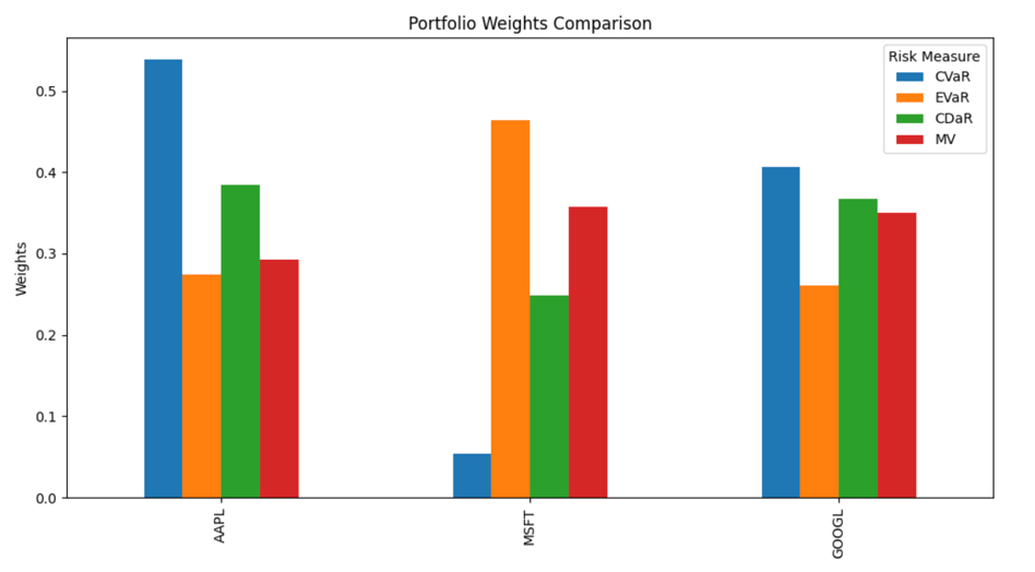
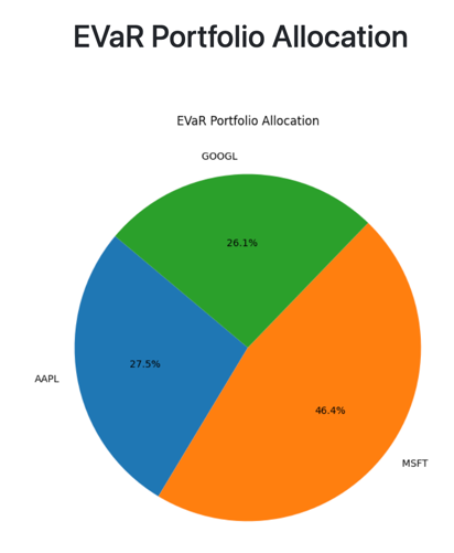
And according to entropic value at risk (EVaR) we, for instance, have following distribution:

Calculating the annual return, annual volatility, Sharpe and Sortino ratio and the max drawdown. All of these metrics are very self-explanatory but:

• The Sharpe ratio is a measure of risk-adjusted return, introduced by William F. Sharpe. It quantifies how much excess return an investment generates per unit of total risk (as measured by standard deviation). $\frac{R_P - R_f}{\sigma_P}$
• The Sortino ratio is a refinement of the Sharpe Ratio, focusing only on downside risk (negative deviations from a target or minimal acceptable return).

EVaR seem to have the highest Annual Return but also the highest max drawdown. Overall CVaR has the best Sortino ratio. Sticking to $P_{CVaR}$ might be the best option.

Usually, we would use a commercial solver for EVaR since its a exponential cone constraints problem. But if we are not willing to pay for that, we could use Deep Learning methods as an approximation.

Conclusion

The Black-Scholes equation for pricing options is derived from Brownian Motion, which is modeled as a random process. This implies that, under the model, the price movements resemble a random walk in continuous price space. This raises the question of whether we can reliably build a portfolio using historical data. For instance, Yang and Ke ⁴ have shown that the Black-Scholes model often deviates from empirical market data. Similarly, Malkiel ¹ argues that detecting patterns in stock charts is often a statistical illusion. This discrepancy between the theoretical underpinnings and real-world results suggests caution when relying solely on past trends for making investment decisions